Real-Time IIR Notch Filter
Audio interference removal using cascaded notch filters on STM32F746
Overview
Designed and implemented dual second-order IIR notch filters to remove interference tones from audio signals in real-time, achieving 30 Hz bandwidth with -3dB attenuation at target frequencies.
Highlights
- Pole-zero placement method for precise notch design at 774.7 Hz and 2231.2 Hz
- Cascaded second-order IIR sections running at 48 kHz sample rate
- Floating-point implementation with Q15 conversion for audio I/O
- Verified performance using network analyzer and FFT spectrum analysis
Tech Stack
Audio Signal Analysis
The input audio file contained two prominent interference tones at 774.7 Hz and 2231.2 Hz that degraded audio quality. DFT analysis in MATLAB revealed these tones as sharp peaks in the magnitude spectrum. The interference frequencies were identified with high precision by examining the DFT and frequency vectors directly, as reading from plots could introduce rounding errors. The 48 kHz sampling rate provided sufficient spectral resolution to accurately locate and target these interference tones.
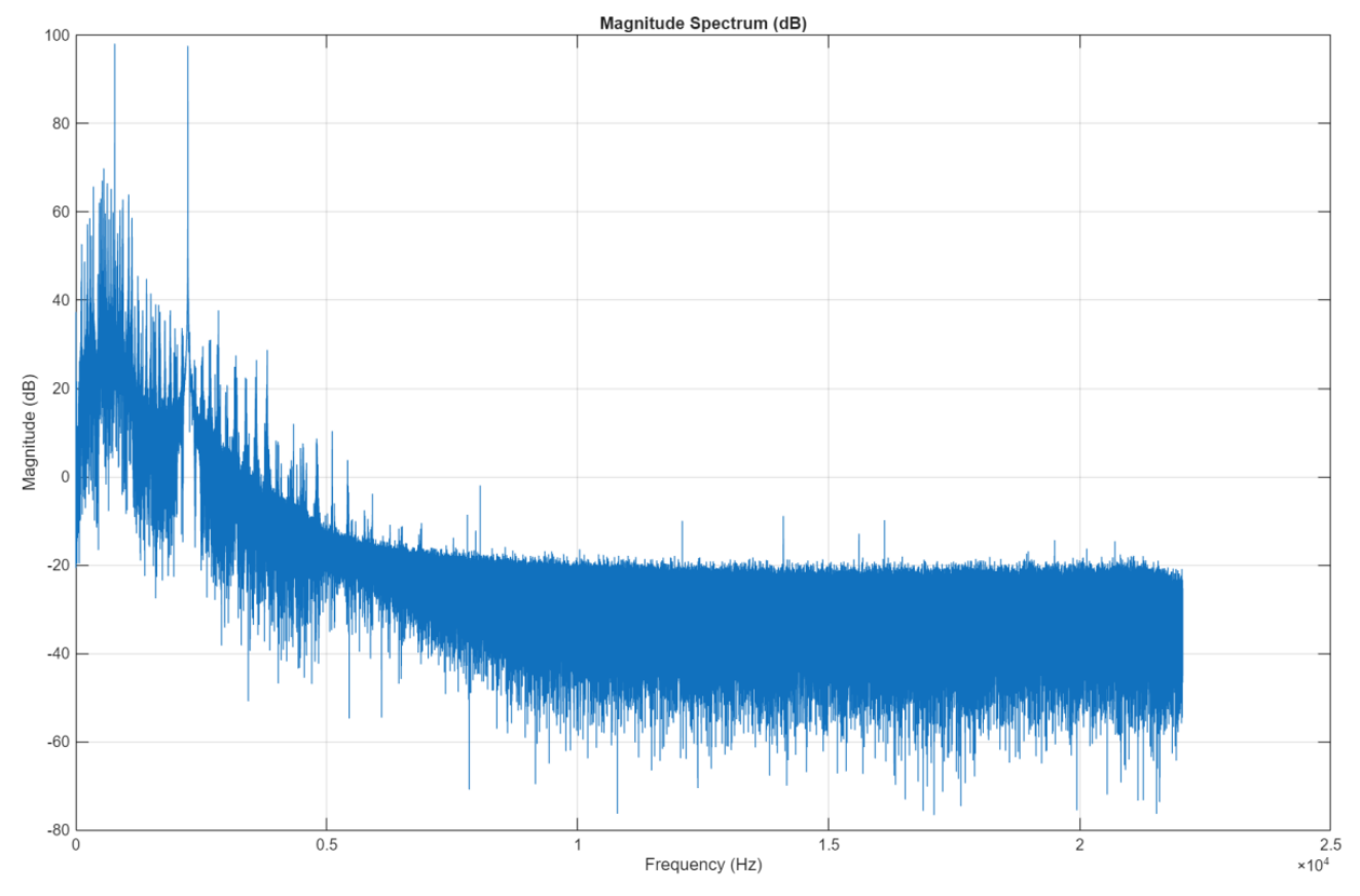
Figure 1: DFT magnitude spectrum showing interference tones at 774.7 Hz and 2231.2 Hz
Transfer Function & Pole-Zero Placement Method
The notch filter design employed the pole-zero placement method with the general second-order transfer function: H(z) = [1 - 2cos(Ω₀)z⁻¹ + z⁻²] / [1 - 2r·cos(Ω₀)z⁻¹ + r²z⁻²] where Ω₀ is the digital notch frequency (radians/sample) and r is the pole radius. The digital frequencies were calculated from analog frequencies using Ω = 2πf₀/Fs. Zeros are placed exactly on the unit circle at angles ±Ω₀, creating complete attenuation at the notch frequency. Poles are positioned at the same angles but at radius r < 1, just inside the unit circle. The pole radius r controls the notch bandwidth - values closer to 1 produce narrower notches with sharper roll-off.
Notch Filter Design - 774.7 Hz
The first notch filter was designed using the pole-zero placement method to remove the 774.7 Hz interference tone. Digital Frequency: Ω₁ = 2πf₁/Fs = 2π(774.7)/48000 = 0.1014 rad/sample Pole Radius (30 Hz bandwidth): r = 1 - (BW·π)/Fs = 1 - (30π)/48000 = 0.99804 Filter Coefficients: b = [1.000000, -1.989725, 1.000000] a = [1.000000, -1.985825, 0.996077] The frequency response shows the notch centered precisely at 774.7 Hz with sharp attenuation exceeding -40 dB.
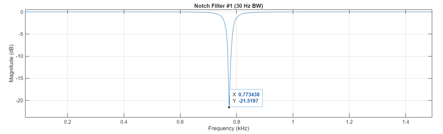
Figure 2: Frequency response of first notch filter at 774.7 Hz
Notch Filter Design - 2231.2 Hz
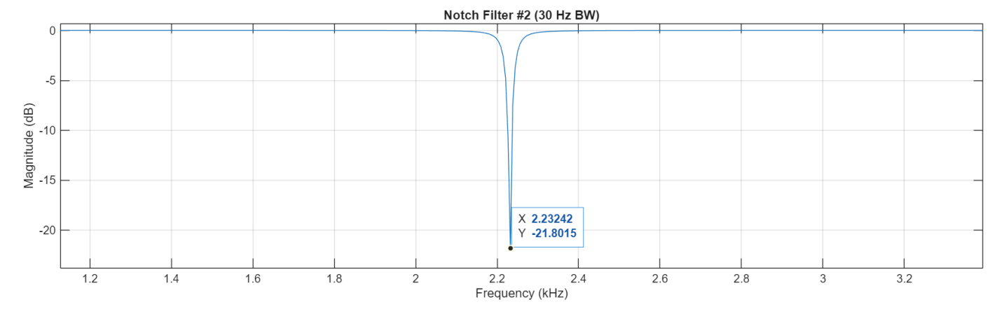
Figure 3: Frequency response of second notch filter at 2231.2 Hz
The second notch filter targets the 2231.2 Hz interference tone using identical design methodology. Digital Frequency: Ω₂ = 2πf₂/Fs = 2π(2231.2)/48000 = 0.2921 rad/sample Pole Radius (30 Hz bandwidth): r = 0.99804 (same as Filter 1) Filter Coefficients: b = [1.000000, -1.915304, 1.000000] a = [1.000000, -1.911554, 0.996084] The frequency response demonstrates sharp attenuation at 2231.2 Hz while maintaining unity gain in adjacent bands. Both filters use identical pole radius values, ensuring consistent 30 Hz bandwidth despite different center frequencies.
Bandwidth Calculation & Verification
The notch bandwidth specification required -3dB attenuation width of 30 Hz. The pole radius r was calculated using: r = 1 - (BW·π)/Fs = 1 - (30π)/48000 = 0.99804 Measured Results: • Lower -3dB point: 759.204 Hz • Upper -3dB point: 790.068 Hz • Measured bandwidth: 30.864 Hz This close agreement with the 30 Hz specification validates the pole radius calculation. The narrow notch design preserves adjacent frequency content while providing deep attenuation (>40 dB) at the target frequencies.
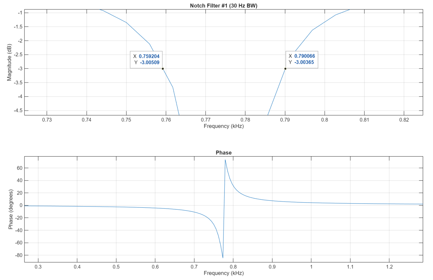
Figure 4: Zoomed view showing 30 Hz bandwidth measured at -3dB points
Pole-Zero Plot - 774.7 Hz Filter
The pole-zero plot for the first notch filter visualizes the strategic placement in the z-plane. Zeros are positioned exactly on the unit circle at angles ±0.1014 radians (±5.81°), corresponding to the 774.7 Hz notch frequency. Poles are placed at radius r = 0.99804 at the same angles, positioned just inside the unit circle. This geometric configuration creates complete attenuation at the notch frequency (where zeros are located) while the nearby poles ensure narrow bandwidth and minimal impact on adjacent frequencies.
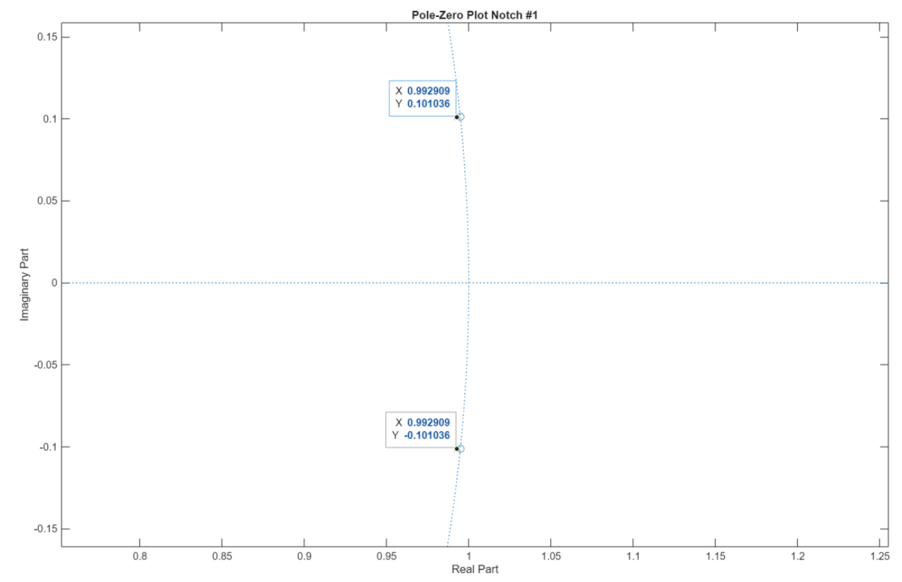
Figure 5: Pole-zero plot showing precise placement for 774.7 Hz notch filter
Pole-Zero Plot - 2231.2 Hz Filter
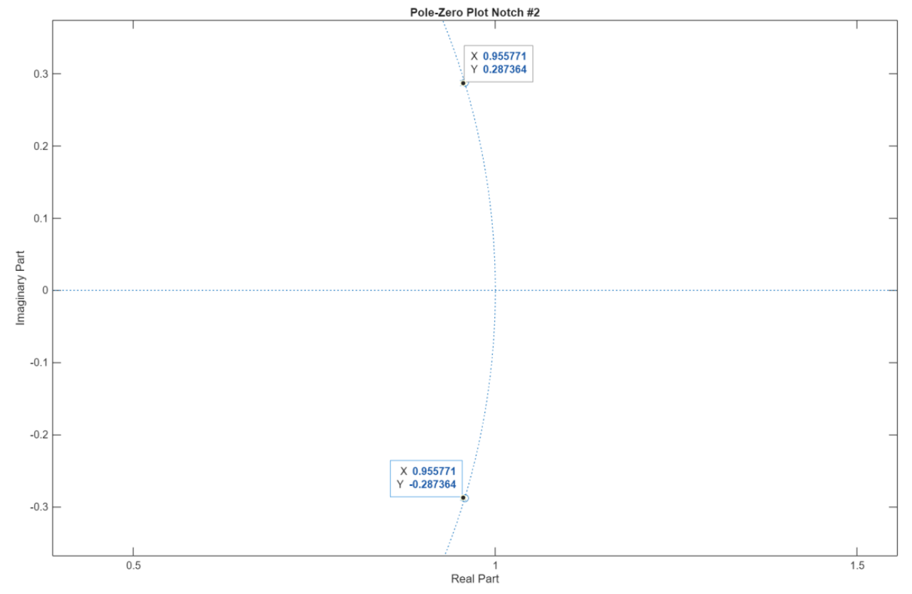
Figure 6: Pole-zero plot showing precise placement for 2231.2 Hz notch filter
The second filter's pole-zero plot shows zeros on the unit circle at angles ±0.2921 radians (±16.73°), corresponding to the 2231.2 Hz notch frequency. Poles are positioned at the same angles but at radius r = 0.99804, just inside the unit circle. The larger angle compared to the first filter reflects the higher notch frequency. Both filters use identical pole radius values, ensuring consistent 30 Hz bandwidth despite different center frequencies. This demonstrates the scalability of the pole-zero placement method across the frequency spectrum.
Real-Time Hardware Implementation
The STM32F746-DISCO implementation used 48 kHz sampling rate with dual-channel processing: LEFT channel provided pass-through audio for comparison, RIGHT channel processed audio through both cascaded notch filters. The C code implemented the difference equations using single-precision floating-point arithmetic (float32_t) for filter calculations. Static variables stored filter states (x1, x2, y1, y2) between samples, maintaining causality. Input samples were converted from Q15 fixed-point format to floating-point, processed through both filters in series, then converted back to Q15 for audio output. The LINE IN connector received audio from a laptop or network analyzer.
Network Analyzer Frequency Response - 774.7 Hz Notch
Hardware verification using the Analog Discovery 2 network analyzer measured the actual frequency response of the implemented filter. The measured response shows the first notch at 766.12 Hz (within 1% of the 774.7 Hz design target) with -3dB bandwidth of approximately 29.3 Hz. The cursors show the -3dB points at C1: -0.44304 dB and C2: -2.84435 dB, with ΔX of 29.282 Hz. This close agreement between measured and designed values validates the MATLAB filter design and C implementation accuracy.
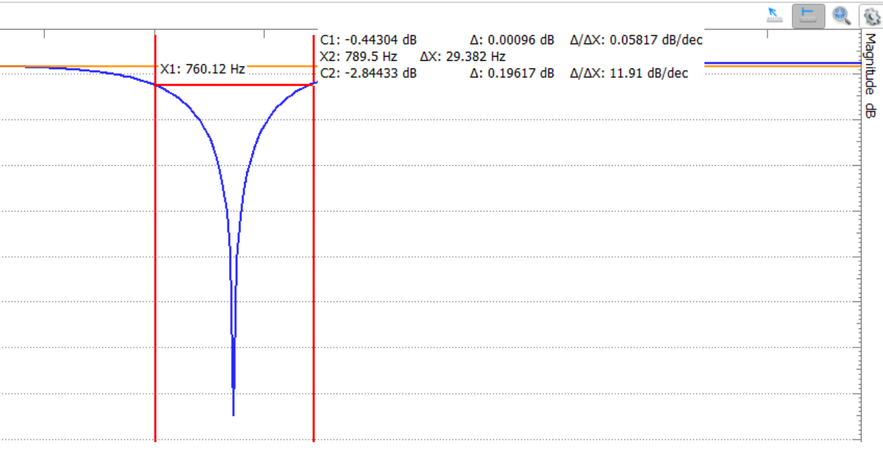
Figure 8: Network analyzer measurement of 774.7 Hz notch showing 30 Hz bandwidth
Network Analyzer Frequency Response - 2231.2 Hz Notch
The network analyzer measurement of the second notch filter shows the notch centered at 2216.3 Hz (within 1% of the 2231.2 Hz target) with measured bandwidth of 30.058 Hz. The measurement cursors indicate X1: 2.2163 kHz, X2: 2.2455 kHz, with ΔX: 29.175 Hz and C2: -2.89774 dB at the -3dB point. Both hardware-measured notches demonstrate excellent agreement with MATLAB predictions, confirming the filters operate as designed on the STM32 hardware with minimal deviation from theoretical performance.
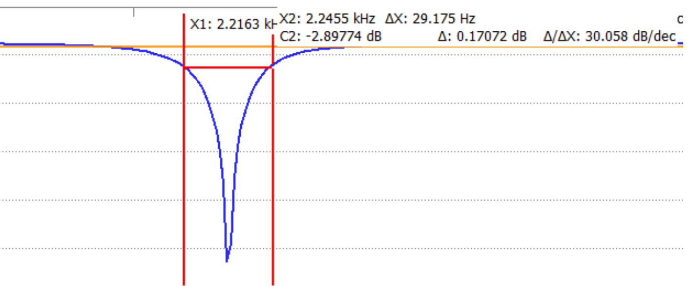
Figure 9: Network analyzer measurement of 2231.2 Hz notch showing 30 Hz bandwidth
FFT Spectrum Analysis - Interference Removal
Real-time FFT spectrum analysis comparing LEFT (unfiltered, orange) and RIGHT (filtered, blue) channels confirmed successful interference tone removal. The LEFT channel spectrum shows prominent peaks at 775 Hz and 2.234 kHz corresponding to the added interference tones. The RIGHT channel spectrum shows these peaks completely eliminated by the cascaded notch filters while preserving all other frequency content. The broadband audio spectrum remains intact, demonstrating that the narrow 30 Hz notches remove only the interference without affecting adjacent frequencies or introducing audible artifacts.
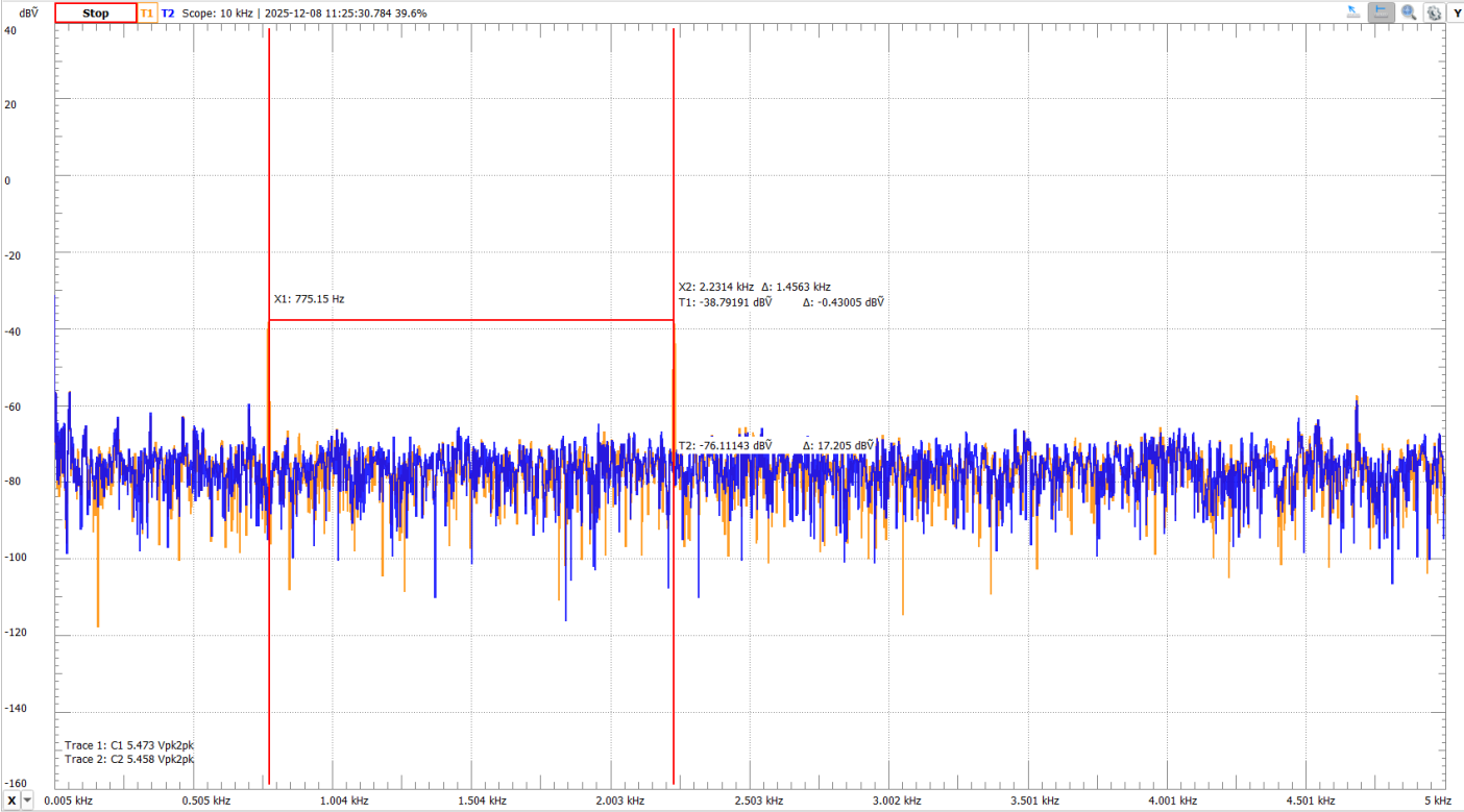
Figure 10: FFT comparison showing complete interference tone removal in filtered channel
Cascaded Filter Architecture
The two notch filters were implemented in series (cascaded) rather than as a single fourth-order filter. This approach improves numerical stability and simplifies coefficient calculation. The output of Filter 1 becomes the input to Filter 2, with independent state variables for each filter preventing cross-contamination. Cascading second-order sections is standard DSP practice for implementing higher-order filters, as it avoids the numerical precision issues associated with direct-form higher-order filters. Each filter maintained its own difference equation and state history.
Key Learnings & Results
- Pole-zero placement method provides intuitive control over notch frequency and bandwidth through geometric positioning in the z-plane
- Cascading second-order sections yields better numerical stability than designing higher-order filters directly
- High-precision filter coefficients (format long in MATLAB) are critical for matching theoretical and measured responses
- Real-time audio processing requires careful management of floating-point arithmetic and state variables in C
- Network analyzer provides accurate hardware verification by measuring relative channel responses
- Notch filters effectively remove tonal interference while preserving broadband audio content and maintaining subjective audio quality